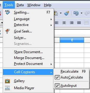
| 1 | To apply conditional formatting, AutoCalculate must be enabled. Click Tools | Cell Contents | AutoCalculate |
 |
| 2 | In your spreadsheet, select the cells to which you want to apply conditional formatting. |  |
| 3 | Choose Format | Conditional Formatting | 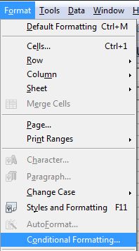 |
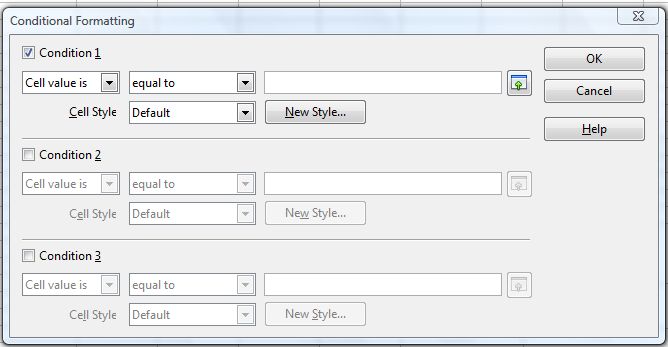
| 4 | On the Conditional Formatting dialog, enter the conditions.
|
|
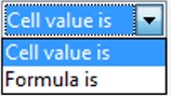
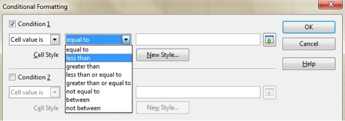
| 5 | Note every condition has several aspects. The cell value is the option usually referred to when constructing a condition. |
 |
| 6 | The value in the cell will either be equal to, less than or greater than (and see the other options) to a certain condition. We will select less than in this example (see below) | 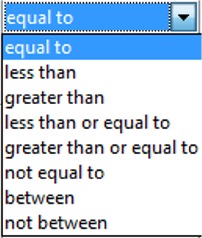 |
 |
||
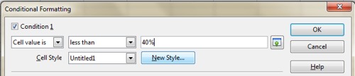
| 7 | The condition is set in the third column - in this case we make the condition 40% (the boundary for a pass and fail)
|
|
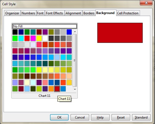
| 8 | We then select the format that should be shown should the condition be met (the statement is TRUE). Click on New Style - the Cell Style popup window appears. In tis example we select a Background (clicked on the Background Tab) and select a red colour. Then Click OK and OK again.
|
|
| 9 | The conditional format rule is now applied and you can see the result (see right) | 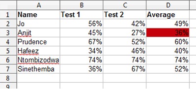 |
Produced by SchoolNet SA